Here's a methodology walkthrough for the Fast, Confident, Wrong business impact model.

This document accompanies the blog post Fast, Confident, and Wrong: The Risk of Noisy Incrementality Tests. The post reports the results; this walkthrough explains how the model produces them, so you can pressure-test the design, adjust the inputs, and rerun everything yourself in the companion spreadsheet.

The model in one paragraph

We simulate a year of experiment-driven marketing decisions for a business whose true channel economics are known and held fixed. Each simulated experiment returns a lift estimate equal to the truth plus random noise, the business reallocates budget based on that estimate, and the process repeats. Because the truth never changes, any difference in outcomes between scenarios comes from exactly three things: how noisy the measurement is, how often the business acts on it, and how large the budget shifts are. Running each scenario 1 million times shows the full distribution of outcomes each approach produces, not just a single lucky or unlucky draw.

The four approaches

The model compares four "incrementality stacks," crossing two levels of measurement quality with two testing speeds. The Monte Carlo Results tab and the blog charts label them:

SE (standard error) is the noise level on each experiment’s measured lift. A 2% SE solution returns estimates tightly clustered around the truth; a 6% SE solution returns estimates that wander, sometimes far enough to make a strong channel look weak, or a weak one look strong.

How one simulated year unfolds

Every simulation run follows the same five steps:

1. Set the ground truth. Eight channels (Meta, Meta Awareness, Google Non-Brand, Google Shopping, Google PMax, YouTube, CTV, TikTok) each get a fixed marginal-return curve. The curve’s shape determines each channel’s true iROAS at any spend level. The business starts by assuming every channel returns the same iROAS; the truth is hidden from it.
2. Run an experiment. A channel is tested in a fixed rotation. The experiment returns a measured iROAS equal to the channel’s true iROAS plus random noise drawn at the scenario’s standard error.
3. Reallocate. The measured iROAS is compared to the running spend-weighted average across tested channels. Budget moves toward channels that look above average and away from those that look below it, capped by the scenario’s reallocation threshold. Money only moves between channels when an experiment has been run and the result supports the trade.
4. Repeat. Steps 2–3 run 6 or 15 times, depending on the scenario’s velocity. Each reallocation changes the starting budget for the next decision, which is why errors can compound rather than average out.
5. Score the year. Final annualized revenue on the true return curves is compared to what revenue would have been with no reallocation at all. That difference is the run’s revenue lift, and it can be negative: with enough noise, "optimizing" leaves the business worse off than doing nothing.

The Monte Carlo grid

One year is one draw of the dice for each experiment. To understand the distribution of outcomes, the supporting script sweeps each of the four approaches across a grid of business conditions and reruns every combination 1 million times:

That is 3 × 3 × 2 × 2 = 36 scenarios × 1 million runs = 36 million simulations. When budgets are scaled up or down across spend levels, each channel’s curve parameters scale proportionally, so starting iROAS stays constant — isolating measurement quality from curve-position artifacts.

What the results show

Three views of the same 36 million runs, all reproducible from the Monte Carlo Results tab.

1. Accurate measurement roughly halves the chance of a wasted year

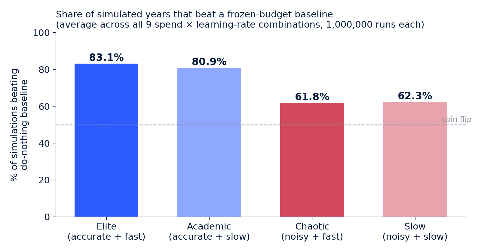
Source: Monte Carlo Results tab, "% Positive" column, averaged across all nine spend × learning-rate cells.

Averaged across every business condition, the accurate approaches beat the do-nothing baseline about 82.0% of the time; the noisy approaches, about 62.0%. Velocity barely moves either pair, which is the core finding: speed cannot practically repair a noisy signal in 1 year.

2. Similar ceilings, very different floors

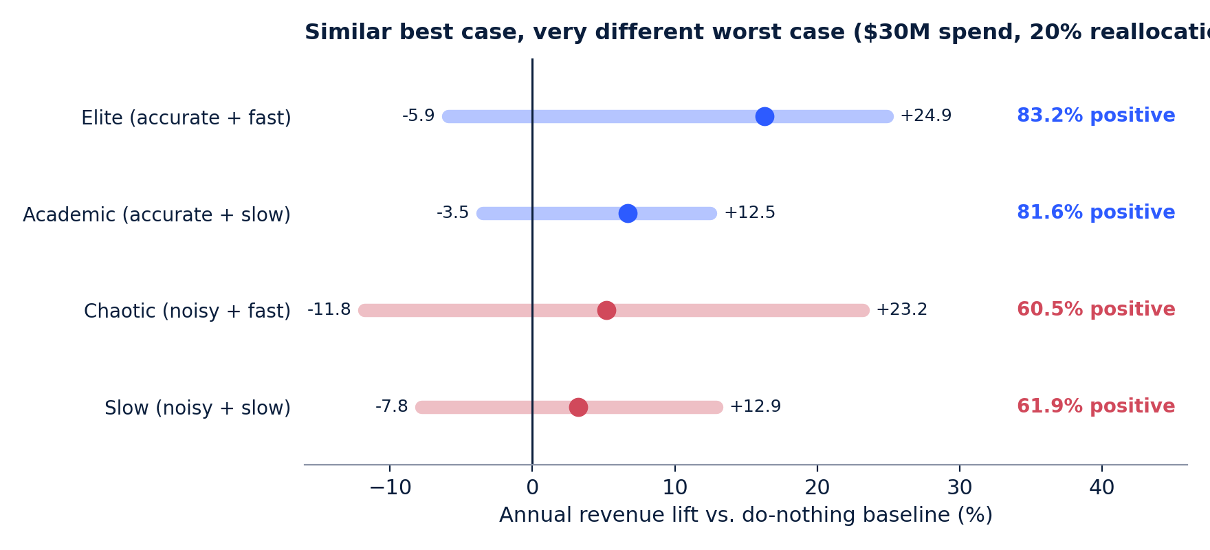
Source: Monte Carlo Results tab, $30M spend / 20% learning rate rows.

In this representative scenario, Elite and Chaotic have similar 90th-percentile outcomes (+24.9% vs. +23.2%). The difference is in the floor: Chaotic’s 10th percentile is twice as deep, and it lands below zero more than twice as often as Elite (39.5% vs. 16.8% of runs). Best-case comparisons hide this entirely.

3. Accuracy earns more lift per unit of risk

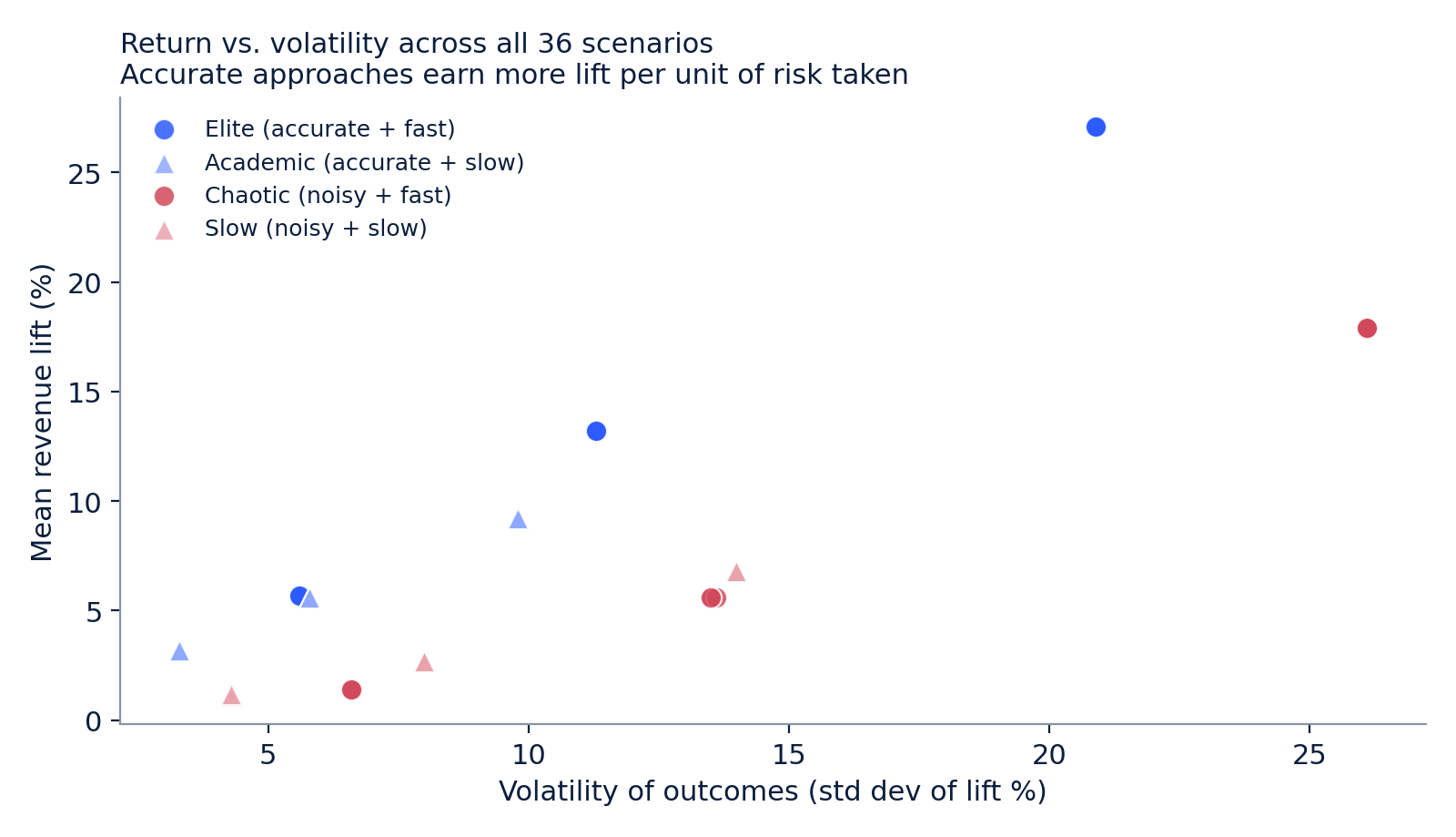
Source: Monte Carlo Results tab, all 36 scenario rows. Mean lift vs. standard deviation of lift.

Plotting every scenario’s average lift against its volatility shows two clean frontiers: at any level of outcome volatility, the accurate approaches (blue) sit above the noisy ones (red). Raising the learning rate moves every approach up and to the right — more aggressive reallocation raises both expected return and risk — but it never lifts a noisy stack onto the accurate frontier.

A guide to the workbook

Assumptions and limitations

The model is a controlled thought experiment, and it is deliberately simple in places. When interpreting the results, keep in mind:

• It models noise only. Measurement quality is represented purely as random error. Systematic bias, unrepresentative market selection, and data-quality failures are not simulated; a real-world noisy solution likely suffers from those too, so the simulated gaps are, if anything, conservative.
• The truth is static. Real channel economics drift with seasonality, creative, and competition. Here they are frozen so measurement quality can be isolated.
• The decision rule is mechanical. Budget always moves after every readout, with no holds, retests, confidence thresholds, or Bayesian partial pooling. A more conservative decision process would narrow (but not erase) the gap between accurate and noisy measurements.
• One year, one rotation. Channels are tested in a fixed order, and the horizon is a single year. Multi-year compounding of good (or bad) measurement is out of scope.
• Channel curves are illustrative. The eight-channel portfolio and its return curves are representative of a DTC media mix, not calibrated to any specific advertiser.

Every input above is adjustable in the workbook. If you think a parameter is unrealistic for your business, change it and rerun — that is the point of shipping the model alongside the post.

‍